
Despite what the movies and television programs may like to say writing computer programs can be very tricky. At the heart of what a computer programmer is trying to do is create a script – typed letters and symbols that a machine can read and then execute as the programmer wanted. For simple starter programs that run on local computers this is quite straight forward. In fact writing local programs for an individual user is a super helpful thing as it allows the automation of repetitive tasks. These are often simple macros that run within an existing piece of software. However for software that will run for lots of people possibly on lots of different computers involving lots of different components then some rules, approaches, methods are needed to stop a single developer getting lost in their own code and to allow multiple developers to work on the same code. This is where computational thinking comes in and is very often the first thing a programmer does before jumping head long into the programming language.
Computational Thinking
Computational thinking is made of three core parts which we will cover in minute but before we do it’s worth taking a step back and thinking why do we need it. Computers are unique in the machinery world as they can do some very clever things very quickly – better than a human can do them. In fact this is the reason why computers are so dominate today – they can think quicker than humans when program correctly. But like any machine if it’s told to do something incorrectly it will just as happily do so. The difference with other machines we can see the moving parts or we can record the pressure or temperature with computers it can be tricky to tell if we have set it up correctly as there are no moving parts – it’s just electricity and magnetism. To help us not make mistakes a way thinking that makes designing, creating, and then deploying computer code is used. That is all computer thinking is – being able to think how a computer will do the thing you want it to do.
Computers: machines to solve problems
First things first – computing thinking is a structure so solve problems which computer is good as solving. This started with mathematical problems in creating accurate results from mathematical functions that humans would make mistakes in. Today computers are still doing mathematical calculations but the outputs won’t be a calculation table but a game or a video player or a webpage. All of the solutions were written in a language that the computer can understand and execute and to get to that we need too know how to program.
The first step is realising that the computer bit is not important. The first thing to realise is what is the problem that we are trying to solve. Many times jumping straight into the programming can feel invigorating in the same way that setting off without a map creates a sense of adventure. Until you get lost, it starts getting dark, you’ve eaten all your food and the phone is dead. So in programming you need to have a map, a plan, a view on how things may fit together to solve the problem. Keep your eye on the prize!
To solve any problem there is a pattern you follow.
- Understand the problem – what is it that we are trying to solve?
- Understand the solution – what specifically at a high level will we produce to solve the problem – the output
- Understand the steps – what will happen to produce the solution
- Understand the proof – what will do to prove the solution is working (repeatable, stable, no side effects)
These four basic steps are what you would do for any problem. The key thing is an identifiable problem and solution that is acceptable. This is different from practicing where you go through lessons to learn how to get better at something. This point is raised as when learning about computers and programming there is a lot of practice to get ready to solve problems so don’t worry if the problems you face are simple. They get hard rather quickly.
Understanding the problem
This may seem like an obvious one but it is amazing how often the problem is either not well understood or the solution not well defined. This is one of the key problems as over time the solution may start to loosen as new options come into play, or the problem goes away, or the problem creates an outcome the solution can not fix (you ran out of time).
Abstraction
Once you have an idea of the problem the next step is to understand what a solution could be at a high level. This means knowing what the outcome of the solution needs to achieve with none of the detail. A simple example would be “I’m hungry. Do you fancy takeaway?” It would be easy to start looking at different take away options, do we pick up or have a delivery, how much money do we have … All of these questions are valid but the high level solution to the problem is not Chinese, India, or fish’n’chips but just food to solve the problem of hunger.
Being able to know the high level goal and parts is called abstraction. An abstract is something that is just the idea of something rather than something that is real. Having and keeping the idea of the solution to the problem allows for a wide view of the problem which is crucial as development starts as problems solved with computers can get complicated quickly.
Abstracting a solution often doesn’t involve any computer programming but is done with paper and pens to create drawings of what needs to be done. The process of abstracting a problem is done in two directions. First the overall problem is stated – “Completing my tax return takes too long”. This can be extracted to a couple of abstract questions that lack detail: what is a tax return, why does it take a long time to fill out. This captures the idea of why a tax return is needed and the idea of filling it in being difficult. From here we can capture the importance of filling in a tax return (you get fined) and it is currently difficult.
Decomposition
With an understanding of the problem and an idea of the big parts of a solution in abstraction we can analyse, investigate, experiment with how the solution would work by breaking the abstract idea down into detail. Breaking some big thing into smaller parts is called decomposition (normally of something rotting but that is not the look we are going for). The reason we break things down into smaller parts is because the code that we write will take in something and then output something else. The change between is the process that the program is written to do. With smaller parts we can define what goes into one part and what comes out. We can link up all the bits to create a single program. Which leads to an interesting point – not all the code we need to write or not all the code will be used as will have to accommodate different scenarios the user of the program may have to do to complete the problem.
An example of this could be our tax return problem of it taking too long. With a single paper form the user may have to fill in all the section in the sections when they only need to fill in a couple of sections and then finish. Another user, with a more complicated life may have to fill the whole form in but they know this so don’t find the form taking a long time to fill in. Note: we have taken the problem of filling in a tax return and created two users who use the form but have different needs. Something to take into account when we are designing the system especially when it comes to how we test it.
Algorithmic Thinking
With a good idea on how we think the solution could work then the next thing is see how the computer can help make the solution. Computers are very, very good at mathematics. Mathematics to many is about sums: adding, subtracting etc. However mathematics isn’t just about arithmetic but about proving truth. This sounds very grand but it’s fundamentally what we are looking to do when we use mathematics – prove and accept that things are what we define them as all the time: 1 + 1 is always 2, anything divided by itself is one. These are both true (you can get funny if you start dividing by zero but let’s not get clever) and proving true or false is called logic or boolean mathematics. Doing arithmetic and testing true or false is the best thing a computer does and this is how we build computer programs. 1) take in something (a parameter), 2) compare it to something, 3) do something based on that comparison, 4) compare the result to something, 5) do something based on that comparison, 6) repeat.
There are two parts to the above: arithmetic and logic comparison. Arithmetic is not just about numbers but anything that we want to manipulate – adding letters to word, subtracting names from a list, multiply pages sent to a printer. Logic operations compare the inputs against a defined condition and then do something depending on the result.
We can use both parts of what a computer is good in our tax form example. Let’s say that if you make less than 10,000 you don’t pay any tax and anything over than is taxed at 10% (if only!).
Please enter your income = ______
income = _____
If income is less than or equal to 10,000 then
   tax = income * 0.0
else
  taxable_income = income - 10,000
  tax = taxable_income * 0.1
print("Your tax is"  & tax & "")
In the above we ask for user to enter their income. We capture this income in a variable called ‘income’. We then check the income to see which tax has to be paid through an “If”. The If checks if the statement “the income level is less than or equal to 10, 000” is TRUE. If is FALSE then calculate the tax as income multiplied by 0.0. If FALSE then do something else in this case take the income and subtract 10,000 then multiply what is left by 0.1 which is 10%. Finally we print out the tax amount to the user that entered the original income.
This is a simple example but contains a lot of the basics when thinking how a computer works. The other thing is looping or iterating through the same code based on a count or a condition.
For the tax form we may need to do an interest calculation on tax that was not paid last year. Keeping things simple let’s say interest on unpaid tax is 10% and a 10,000 bill has not been paid for three years. We can calculate this in two ways: 1) 3 calculations or 2) 1 calculation done three times.
tax_owed = 10000
interest_rate = 0.1

# year 1
tax_interest = tax_owed * interest_rate
total_owed = tax_interest + tax_owed
print(total_owed)

# year 2
tax_interest = total_owed * interest_rate
total_owed = tax_interest + total_owed
print(total_owed)

# year 3
tax_interest = total_owed * interest_rate
total_owed = tax_interest + total_owed
print(total_owed)
This is fine and gives us the answer
11000.0
12100.0
13310.0
This is nice and clear but it’s very wordy and tricky to manage if there are lots of years. The alternative is to use a loop.
tax_owed = 10000
interest_rate = 0.1
years_owed = 3

for i in range(years_owed):
    tax_owed = tax_owed + (tax_owed * 0.1)
print(tax_owed)
This gives the same answer of 13310.0 but it’s a lot cleaner. You may be able to understand how the program works but if you don’t we go through loops in programming fundamentals.
The use of arithmetic, logic decision (True/False) and iteration (loops) are the fundamentals of creating algorithms which make up computer programming.
Algorithms: designing, creating and refining algorithms
For some just the mention of algorithms is a bit daunting just it is important that we understand what we mean when we say algorithms as you are not going to come across the word outside of computers or mathematics.
This may be a bit of a surprise but you probably algorithms already in your life. An algorithm is a set of defined instructions that are produce a known output based on known inputs – the key difference between other processes is there is no deviation from the outputs.
If we take making a cake as an example. This takes known inputs (ingredients), process (recipe) to produce a cake. However every cake will be slightly different as the ingredients will be slightly different, the weight slightly different, temperature of the oven slightly different. You get the idea. The output is slightly different.
With algorithms the input, process, and output is always the same. The most common algorithm you may see everyday is time through digital watches (mechanical watches and clocks get close but springs, weights and other components change over time). Machines that are binary are setup up to run algorithms.
Algorithms can get complicated as there can be multiple inputs, lots of different logic decisions made based on the inputs and other settings. This is where the computational thinking comes in handy: understanding the problem, abstracting the key parts of the problem, decomposing the problem into solutions.
Inputs, Processes, and Outputs
With an understanding of what algorithms are and what they do let us start looking at building one. The first thing to do is to identify the inputs that are needed, a potential high level processes or plan, and the outputs that would be acceptable to the person with the problem. There are several methods that help us capture these inputs, process, and outputs. For our tax problem we know the input is the income and we know the output is the amount of tax owed having gone through the process of multiplying the taxable income by out tax rate. With this information we can start to design a computer program on how this can be taken on (ignore the code from before – we are starting afresh).
Structure Chart and Diagram
One of the basic methods to see how a problem can be viewed is through breaking it down into smaller parts so that it’s clearer what we are trying to do to solve the problem. This is decomposition that is a fundamental part of computational thinking. Breaking down a big thing into smaller bits is all about understanding the structure of the solution.
There are many to break down problems depending on the type of problem. An initial method is brain storming where the problem is broken down into just about anything to try and understand the problem from different views. Brain storming and other methods look to define large areas of the problem that need to be understood to reach a solution.
Once a high level view has been achieved or the problem is simple the problem can be broken into a design or structure where each element is defined as to what it does and how it relates to the other elements.
In computer science we can start with this structured decomposition through structure charts and structure diagrams. Both are related so can be confusing so let’s have a look at each one in turn.
A structure chart is very straight forward: state the problem and then break this down into steps that are needed to solve the problem stated. In our tax problem a structure chart would look like this.
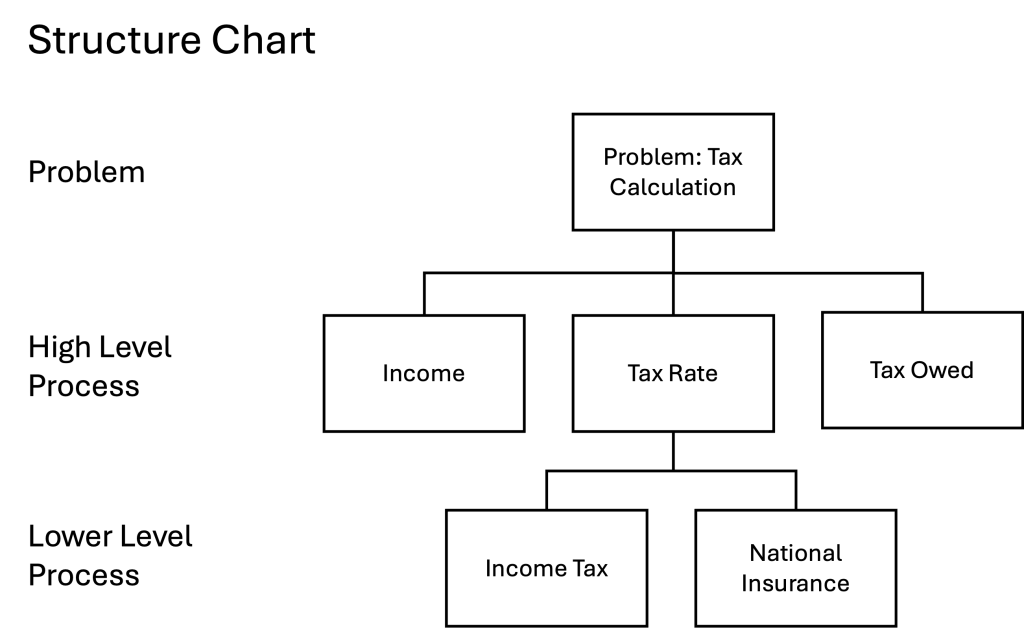
With structure charts you start with the problem at the top. This is then broken down into smaller problems or solutions at different levels. For our simple tax example we have three actions we need to do to calculate the tax that is needed on a certain income. We’ve expanded the problem to have a tax rate that is a combination of two taxes that apply to income. These are shown as a breakdown of the tax rate on a lower level to show how the tax rate is calculated. If there was only one tax rate we would not need to do this. Conversely if the income tax was made of different rates then this could be broken down further. At this point we have not added any specific detail just the major elements that are needed to solve the problem. It is crucial with a structure chart that it is simple and hierarchical so we can change it is necessary. Keeping things simple and true is crucial to algorithmic design.
From this chart we can use a structure diagram which has defined symbols.

For the simple tax calculation the structure chart and structure diagram look the same as the boxes for the chart are the same for the process in the diagram. To give a bit more detail on how the structure diagram works the tax and fine calculation works better. In this diagram we take the tax owed and the apply a fine for every year that the tax hasn’t been paid. As there could be multiple years that tax and the fine could be owing we use the loop symbol. The loop symbol is high level just to show that some process could have to run more than once.
Structured charts and diagrams are very helpful to break the problem into very rough blocks that can be checked easily before getting stuck into the coding detail. Good design saves time.
Flowcharts
The structure chart and diagram give a good high level look at the problem which is a good start. The next thing we can do is look at how data will change as it goes through the program. To show the data flow a flowchart (flow chart) is very helpful.
Flowcharts are used in many forms of analysis to show how things do or could work in the future. Business and process analyst use the same process of how things from how a customers buys a product to how the product is made in the first place. In computer science flowcharts focus more on how the program has to run in order to produce the solution.
Flowcharts are used to show how a process works from start to end. Like the structure diagram it uses symbols to depict what happens at a certain part of the process. There are a couple more symbols to be aware of – one of the key symbols is the diamond which shows a decision point from an input. These are the common flowchart symbols and the tax income calculation and tax owed fine calculation:
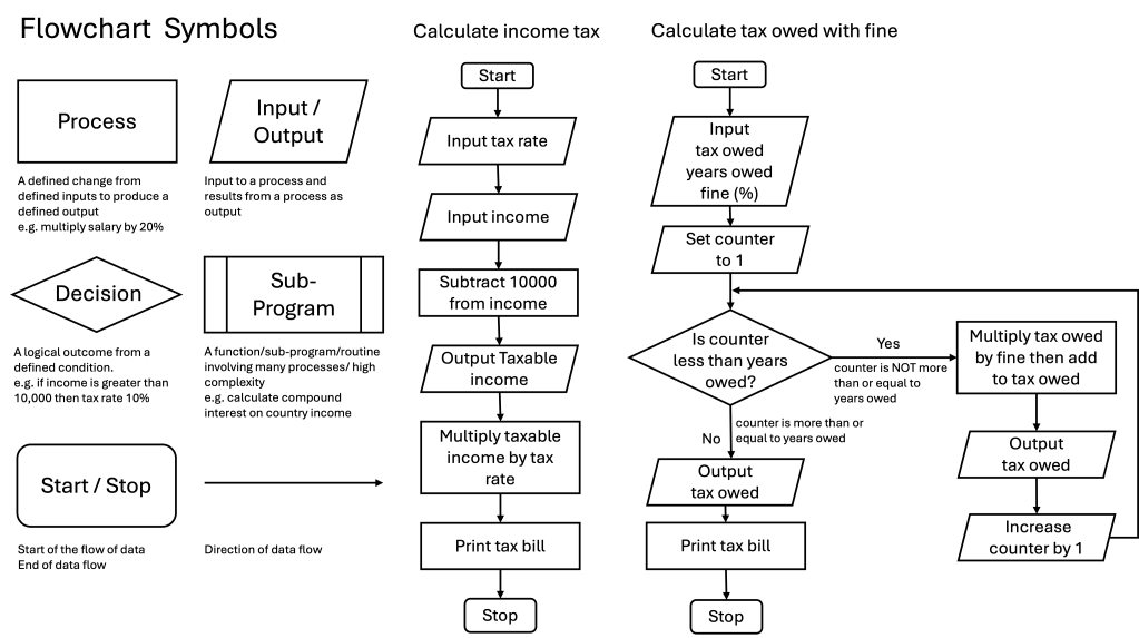
As you can see the flowchart has more detail than the structure chart and the structured diagram and is easy to see how the process will work. The flowchart is similar to the structure diagram in that it has the two core processes of a computer: arithmetic and logical decision making. The difference between the structure diagram and flowchart is the direction of the data is clearer so it’s easier to see what goes into the process and what comes out.
Due to the direction of the data flow is well suited to how computer programs its good to get used to using flowcharts to describe how the program will work for a person and how that is reflected in the code. For example from a person’s point of view trying to buy something on an online shop can be done in many ways: they can browse first, add things to their basket, then checkout; or they may want to log in first to show what they have bought first and then browse. These user journeys can be recorded as flowcharts and then the computer program is created to allow them to happen.
Pseudocode
Great! Structure charts and diagrams along with flowcharts do a lot of the computational thinking before we write any code. But you want to learn how to write algorithms and so will need to know how to do that (after the charts, diagrams, flows etc). Before we break open the IDE (the software you will use to write the software) there is a step between design and code – pseudocode. Fake code?
Pseudocode is not a real programming language as, like linguistic language, they have set of words, rules, structures and other forms of syntax that make them understandable to other people that understand how to listen or read that language. But like all languages there are overarching common rules that they all share. For example in all spoken languages there are names or labels for things – computer, human, chair, etc; there are doing words – eat, sleep, run, etc, and there are describing words – quickly, big, under, etc. This is what pseudocode is – a simplified computer language that has the general shape that someone with computer programming experience can understand even if they know different languages.
There is no strict way to write pseudocode but there are ways that everyone accepts as being helpful. For example telling (or declaring) variables that will store data in the program at the begin is helpful so you can when all in one go. Using descriptive labels for variables is also good to make them easier to understand. “Tax Owed” could be written simply as TO to save on writing or even tO to make it even more difficult to understand but in pseudocode the idea is to lay it out in a common structure.
There is catch 22 with pseudocode: how do you write pseudocode with out knowing a programming language? The answer is actually quite easy – in bits (no pun intended). To start to write in pseudocode you have to be able to explain the problem and what the outcome you want. The second thing you need to do is break the problem into input, processes, outputs, loops, and decisions. The third, and last thing, is to know the basic components of a computer program. We know the first two what about the third?
We cover the fundamentals of programming to give more specific details on how to write a program but we can give you a cut down version to explain pseudocode.
- Declare variables to store inputs, outputs and counters
- Capture counted loops (ones that run for defined number of times)
- Capture conditional loops (ones that run until a condition is meet – true or false)
- State decisions conditions and options on decision outcomes
- Correctly format structure common to computer code (comments, indentation, capitalisation)
Breaking this down for our tax examples
# Calculation of tax

input income
input tax_rate

tax_owed = income * tax_rate
print tax_owed
This is a super simple example and it’s good start as you can (hopefully) see how you could write with this in any programming language. For the tax fine algorithm it’s still straight forward
# Calculation for outstanding tax owed with yearly fine

input tax_owed
input years_owed

fine_interest_rate = 0.1

loop for years_owed:
    tax_owed = tax_owed + (tax_owed * fine_interest_rate)
print(tax_owed)
In this example we take in two variables and set (hardcode) a variable then we say to loop the following code for the number of years outstanding adding the fine to the tax owed for each year before printing the amount an individual owes.
Reference language/high-level programming language
The next step after pseudocode is to use a reference language which is a stricter form of pseudocode which contains an agreed structure and syntax. A reference language contains all the elements you will find in most programming languages which we cover in programming fundamentals. The need for reference language is special important when working in languages that are nearly impossible to read without training in the language.
Searching and Sorting Algorithms
To start to learn algorithms there are two very common algorithms that computers are very good at (and humans are bad at at scale): 1) Sorting data, and 2) Searching data. We’ll look at each and show how using computational thinking you can understand how to build algorithms.
Note: don’t worry about the mathematics for now (understanding and practice
The first thing to recognise when looking to create algorithms is not panic about any mathematics. You will come across terms like n+1 or n^2 to show how the algorithm works with respect to the number of times it has to run in order to complete its function. Let’s take it nice and slowly (as this is the best way) to understand what the computer is doing.
Sorting
Picture the scene: you have a load of different value coins that need sorting in order from lowest value to the highest. For a human to do this it is easy – we look at the coin assess its value then place it down. We then pick up another coin assess its value and place it to the left or the right of the previous coin. We repeat this until all the coins are placed in order from highest to lowest. Easy. Now imagine there are a million coins that need sorting. The process is the same but it has two challenges: 1) errors (accidentally placing a coin in the wrong order) and 2) time (it would take a very long time to sort all the million coins!). Errors and speed are two reasons why we have machines – they take the load of humans who are limited by their own biology. To sort a million coins we could build a machine that can assess the coins and sort them based on that assessment. The machine would be programmed to do what we instructed and its the instruction where the algorithm sits – a repetitive instruction.
There are three basic sorting algorithms that are taught at GCSE level to show how algorithms can be used to sort a list of numbers. Each sorting algorithm does the same thing but they do it in different ways. The same thing is what we would do: compare two things and then swap them if they were different – they just do it very quickly.
It’s worth noting that you will (probably) very have to write a sorting algorithm as the programming languages have built in functions that do this already.
For the examples we will use we are sorting a set of numbers into a list for low to high but we could change the algorithm to do the opposite as the computer doesn’t care.
Bubble Sort
The first sort has the friendly title of bubble sort as the high numbers at the bottom of the list bubble up to the top like bubbles in water. The first thing to do is write out the simplest case so you can picture how it would work (if you are super smart then you can jump ahead to the maths).
List – 2 values
The simplest list would be 2 numbers: 34, 95
Although there are are only two numbers there’s more information here that we’ll use in all the sorting and searching algorithms. Lists have a length (number of values in the list) and values in the list have a position. The positions of those values are both absolute and relative. Absolute values are the number in the list (number 3 is the queue) and relative values (number 3 is after number 2 and before number 4). The length and position of things in the list is important for sorting as the things in the list are not often numbers but words. For example a list of name of students that you want to sort alphabetically.
As humans when we look at a list we number it like this
| List Position | 1 | 2 |
| List Value | 36 | 94 |
If asked where in the list is position 36 you’d say at position 1 and 94 is at 2 or next to 36. Labelling where things are relative to another thing in an order is a called an index. In a book an index is a list of terms in alphabetical order. Labelling positions 1 and 2 is indexing the list. We can index a list in anyway we want but we normally start at one. With computer programs we can start at zero or one. The most common programming (Python, C, C++, Java) use zero as the starting value. Starting our paired list at zero we get the following.
| List Index | 0 | 1 |
| List Value | 94 | 36 |
Why does it matter starting at zero? The advantage is in this list we don’t care about the count but the position of values. 94 is not the second value in the list; it is the first one after the initial value. It is +1 away from the start. To get to 96 move +1 up from 36. For the above list the length is 2 and it has values from position 0 to 1.
With this information we can start to look at the logic to sort this list. For our example list the logic would be:
If value at index 0 > value at index 0+1 is True then:
value at index 0 = value at index 0+1
value at index 0+1 = value at index 0
else (index 0 < index 0+1):
end
If we run this through our example list:
If 94 > 36 is True then:
94 = index 0+1
36 = index 0
else:
end
This leaves the list looking like this
| List Index | 0 | 1 |
| List Value | 36 | 94 |
The list is now sorted from lowest to highest in terms of number size. If we look at the list vertically instead of horizontally then you can see why it’s called a bubble sort.
| Index | Value |
| 1 | 36 |
| 0 | 94 |
-> swap “bubble”
| Index | Value |
| 1 | 94 |
| 0 | 36 |
This makes sense for a human but there is a problem for a computer. We can’t swap the values in two steps as we’d be referencing the change just made so we have to do it at the same time. The python code for this swap looks like this:
# Before swap
list_1 =[94, 36]
print (list_1)
print(list_1[0])
print(list_1[1])

if list_1[0] > list_1[1]:
    list_1[0], list_1[1] = list_1[1], list_1[0]

print("---")
# After swap
print(list_1)
print(list_1[0])
print(list_1[1])
The result looks like this:
[94, 36]
94
36
---
36
94
36 is now at index 0 and 94 is at index 1. If we ran this again nothing would happen as 36 is less than 96 so the if statement would be false. 94 bubble up above the lower 36. The reason for the bubble up instead of sink down is the focus is on the larger number moving up rather than the other value going down.
We’ll see this bubble effect when we look at a long list than 2. Let’s look at a list of 3. Again, this may seem like a very slow explanation but stick with it as it’s going to start to get more complicated as we have a list more than 2.
List 3 numbers
Let the list now be 94, 36, 5. Let’s put this in table to show the values and index
| List Index | 0 | 1 | 2 |
| Index from 0 | – | +1 | +2 |
| List Value | 94 | 36 | 5 |
Lets apply the code we used for the 2 value list
If value at index 0 > value at index 0+1 is True then:
value at index 0 = value at index 0+1
value at index 0+1 = value at index 0
else (index 0 < index 0+1):
end
This will sort the first two value (index 0, index 0+1) 94 and 36. It’s easy to extend this to handle the third value as we can repeat the if statement.
If value at index 0 > value at index 0+1 is True then:
value at index 0 = value at index 0+1
value at index 0+1 = value at index 0
If value at index 0+1 > value at index 0+2 is True then:
value at index 0+1 = value at index 0+2
value at index 0+2 = value at index 0+1
The python for this is
list_2 =[94, 36, 5]
print (list_2)

if list_2[0] > list_2[1]:
    print("It is bigger - swap")
    list_2[0], list_2[1] = list_2[1], list_2[0]

if list_2[1] > list_2[2]:
    print("It is bigger - swap")
    list_2[1], list_2[2] = list_2[2], list_2[1]

print("---")
print(list_2)
The result looks like this:
[94, 36, 5]
---
[36, 5, 94]
94 has bubbled up two places. All good. Now we sorted the highest value to the top we need to run it again to sort out the 36 and the 5. This gives us a program to sort three numbers:
list_2 =[94, 36, 5]
print (list_2)

if list_2[0] > list_2[1]:
    list_2[0], list_2[1] = list_2[1], list_2[0]

if list_2[1] > list_2[2]:
    list_2[1], list_2[2] = list_2[2], list_2[1]

if list_2[0] > list_2[1]:
    list_2[0], list_2[1] = list_2[1], list_2[0]

print("---")
print(list_2)
The result looks like this:
[94, 36, 5]
---
[5, 36, 94]
Excellent – we can now sort a list of three numbers.
However, you may be starting to think a couple of things: 1) can we reuse the code that we have already written as we repeat the same thing twice? 2) how do we cope with a very long list of values – this won’t work with even 10 number. Is there a smarter way of doing this?
Yes! We need to look at this problem as a mathematical problem but don’t panic if maths is not your thing. Again taking things slowly is the key here (as we’re not great at maths to be very honest).
How many times will a number by sorted?
Our first problem with writing a lot of repeating code is knowing when to stop. We could (could) write a 100 if statements to swap values around and a) hope the list is less than a 100, b) hope the computer could cope with it, c) no one ever sees our code. For the bubble sort what is the maximum number of times that a value can be swapped (bubbled) with its neighbour? Let’s work it out.
| List Length | 0 | 1 | 2 | 3 | 4 | 5 |
| Number of swaps | – | 0 | 1 | 2 | 3 | 4 |
| Diff length – swaps | – | 1 | 1 | 1 | 1 |
So the maximum number of swaps needed to get a value from the bottom to the top is the length of the list -1. Easy. This is the number of times we would have to make sure that the highest value bubbled (swapped) to the top (right side) of the list.
Knowing how the maximum number of swaps for list is the first part of getting our algorithms to repeat, or loop, itself. We can now add a for loop (as we know how many times it will run) to our code so the code can be repeated until the condition is no longer true – in this case when the for loop runs out.
We can work out the list length by using a pre-defined algorithm or function that gives the length. In python this is the function len (shortened version of length) which we will use to give the length of the list defined as list_length. Knowing this we can use to set the number of times the loop will run to swap pairs of values to make larger values bubble up.
The for loop also gives us a helpful counter that is used to count the number of times the loop has run. At their simplest for loops are set with a maximum number of times they will loop. Every time they complete a loop the counter is increased by one starting at zero. This counting is the same for the index of the list so the value can be substituted allowing a direct reference to the list index on each loop.
| For Loop Counter Value | List Index Value | List Value |
| 0 | 0 | 5 |
| 1 | 1 | 4 |
| 2 | 2 | 3 |
| 3 | 3 | 2 |
| 4 | 4 | 1 |
As the loop counter is the same as the index we can substitute the for loop counter value for the index value of the list. We can test this by printing the values of the for loop counter and the index list. For loops we general define the counter as the letter i ‘eye’ . In the code below because we are writing letters the number has to be converted to a string through wrapping in the str function.
list_3 = [5,4,3,2,1]
list_length = len(list_3)
print(list_length) # 5
print("---")
for i in range (5):
    print("For loop counter value: " + str(i))
    print("List value at index same as loop counter: " + str(list_3[i]))
The result looks like this:
For loop counter value: 0
List value at index same as loop counter: 5
For loop counter value: 1
List value at index same as loop counter: 4
For loop counter value: 2
List value at index same as loop counter: 3
For loop counter value: 3
List value at index same as loop counter: 2
For loop counter value: 4
List value at index same as loop counter: 1
Now we know we can substitute the list index value for the loop value we can write the swapping condition and the swap as reference to the loop not the list index. This means the loop and the swap is linked so we can sort the first number from the list to the top. Here is the code for that along with a print of the loop counter to show you the value for each loop.
list_4= [5,4,3,2,1]
list_length = len(list_4)
print(list_4)
print("---")
for i in range(list_length - 1):
    print(i)
    if list_4[i] > list_4[i+1]:
        list_4[i], list_4[i+1] = list_4[i+1], list_4[i]
        print(list_4)
print("---")
print(list_4)
The result looks like this (the 5 has been bolded):
[5, 4, 3, 2, 1]
---
0
[4, 5, 3, 2, 1]
1
[4, 3, 5, 2, 1]
2
[4, 3, 2, 5, 1]
3
[4, 3, 2, 1, 5]
---
[4, 3, 2, 1, 5]
Awesome! We’ve now sorted the first number. But how do we do the other numbers? We could repeat the above code for the number of values in the list minus one as the last one will have been sorted if all the other ones are in place. To simply repeat the code for the second number isn’t that crazy an idea. For example if we run the above code for our list 5,4,3,2,1 after 4 rounds the list will be sorted
list_4= [5,4,3,2,1]
list_length = len(list_4)
print("---1")
print(list_4)
for i in range(list_length-1):
    if list_4[i] > list_4[i+1]:
        list_4[i], list_4[i+1] = list_4[i+1], list_4[i]
        print(list_4)

print("---2")
print(list_4)
for i in range(list_length-1):
    if list_4[i] > list_4[i+1]:
        list_4[i], list_4[i+1] = list_4[i+1], list_4[i]
        print(list_4)

print("---3")
print(list_4)
for i in range(list_length-1):
    if list_4[i] > list_4[i+1]:
        list_4[i], list_4[i+1] = list_4[i+1], list_4[i]
        print(list_4)

print("---4")
print(list_4)
for i in range(list_length-1):
    if list_4[i] > list_4[i+1]:
        list_4[i], list_4[i+1] = list_4[i+1], list_4[i]
        print(list_4)
print("---Final List")

print(list_4)
The results look like this
-START--1
[5, 4, 3, 2, 1]
[4, 5, 3, 2, 1]
[4, 3, 5, 2, 1]
[4, 3, 2, 5, 1]
[4, 3, 2, 1, 5]
---2
[4, 3, 2, 1, 5]
[3, 4, 2, 1, 5]
[3, 2, 4, 1, 5]
[3, 2, 1, 4, 5]
---3
[3, 2, 1, 4, 5]
[2, 3, 1, 4, 5]
[2, 1, 3, 4, 5]
---4
[2, 1, 3, 4, 5]
[1, 2, 3, 4, 5]
---Final List
[1, 2, 3, 4, 5]
This may seem like a barmy idea to just keep repeating the code but it’s another step to seeing how we could improve it. It’s better to get working inefficient code than keep trying fancy code that doesn’t work.
What we can see from the code above is we need another loop to go through all the positions in the list to check if a value is higher so it can bubble to the top. From the code above it took 4 loops to sort the 5 item list. The reason for 1 less than the total length is the last item does not need to sorted as it has sank to the bottom. This is not ideal as we will want to check the list has no swaps so an extra loop is good to use the length of the list. This makes sense if you had a list of 4 numbers you’d have to check the 4 positions to see if they needed swapping.
Putting this outer loop does t
list_5 =[9,8,7,6,5]
list_length2 = len(list_5)

print("--- Unsorted ---")
print(list_5)
print("---------------")

for i in range(list_length2):
    for j in range(list_length2 - 1):
        if list_5[j] > list_5[j+1]:
            list_5[j], list_5[j+1] = list_5[j+1], list_5[j]
            print(list_5)

print("--- Sorted ---")
print(list_5)
print("---------------")
The result looks like this …
--- Unsorted ---
[9, 8, 7, 6, 5]
---------------
[8, 9, 7, 6, 5]
[8, 7, 9, 6, 5]
[8, 7, 6, 9, 5]
[8, 7, 6, 5, 9]
[7, 8, 6, 5, 9]
[7, 6, 8, 5, 9]
[7, 6, 5, 8, 9]
[6, 7, 5, 8, 9]
[6, 5, 7, 8, 9]
[5, 6, 7, 8, 9]
--- Sorted ---
[5, 6, 7, 8, 9]
---------------
Wow! We have written an algorithm that sorted the list. Now, it won’t be the best way of doing this and there will be better, more sophisticated ways of doing this but the principle will be the same: iterate through the numbers horizontally looking for swaps starting at the first index location, once all swaps done then repeat starting at the next location in the list.
An algorithm that takes in a defined input and does one thing we can capture as a function. By capturing an algorithm as a function we can use is over and over. A quick introduction to functions:
def bubble_sort(list): # this is the name of the function and what it takes in
# for python the indentation is important to score the contents of the function
    list_length = len(list)

    print("--- Unsorted ---")
    print(list)
    print("---------------")
    for i in range(list_length):
        for j in range(list_length - 1):
            if list[j] > list[j+1]:
                list[j], list[j+1] = list[j+1], list[j]
                print(list)
    print("--- Sorted ---")
    print(list)
    print("---------------")

# that's the end of the function.

# Two list for the bubble_sort to work on
list = [6, 5, 4, 3, 2, 1, 0]
test_scores = [60, 85, 41, 30, 12, 95, 0]

# Feed the function. It doesn't matter what you call it as long as it's a list (or whatever the function can process

bubble_sort(list)
bubble_sort(test_scores)
The results work like above so we won’t show the results. Try it and you’ll see it how it works.
Merge Sort
The bubble sort is probably the easiest sort to work out as it pretty straight forward swapping higher numbers for lower numbers in pairs until sorted. The problem with this approach is that it does not work well for very long lists as you have to keep going back to the very beginning every time. For long lists that need sorting there is a more complex method that makes better use of what a computer is good at: repeating things over and over.
Imagine you have a very large list of numbers say 1000 and you wanted to sort them from lowest to highest values. The bubble sort would do this but it would have to go through 1000 loops to be sure. A better way of sorting large lists is with a bit of overhead that offsets the linear sorting like a bubble. That overhead is to split the list and then sort smaller lists. This is what the merge sort does. It would be more helpful to perhaps call it the “split and remerge” sort as there are two parts to this sorting algorithm. Again we’ll start super simple and build up the complexity. Just remember the merge sort is for big lists due to the order head of the split. The split and merge is sometimes called divide and conquer which you will see in the search algorithms.
The merge sort takes a list and divides it into two smaller parts until there are individual items to be compared. Let’s start with 2 values.
list =[2, 1] – remember this list is 2 long having an index of 0 and 1 in python (other languages start their index at 1 rather than zero)
First – split the list in half into two lists half the size. Keep splitting until the list is in single lists.
Second – rebuild the single lists into first pairs. Then compare the pairs to build a 4, then an 8. until the list has been rebuilt. Easy.
list_1 = [2,1]

index  [0][1]
values [2][1]
split - create 2

       list_1-1 list_1-2
index  [0]      [0]
values [2]      [1]

Can the list be divided any further (is the length greater than 1)?
No - start compare and merge!!!

Is value at position 0, list_1-1 greater than value at position 0, list_1-2?
if yes swap values in the two lists

merge two lists into one list
list_1 = [1,2]
You can see that this is way more steps than the bubble sort to pretty much do the same thing swap to values. True. The reason we use it is for longer list. Say 3 values …. and this is where we need a little thinking. Let the list be 3, 2, 1.
We have split the list into 3 lists
# indentation is to show the relationship

                Level 0                   list_1 = [3,2,1]

index                                           [0][1][2]
values                                          [3][2][1]
split - create 2

                Level 1      list_1-1               |        list_1-2
index                        [0][1]                 |          [0]
values [3,2]                 [3,2]                  |          [1]

Can the list be divided any further (is the length greater than 1)?
Yes

                Level 2 list_1-1-1  | list_1-1-2
index                         [0]        [0]
values                        [3]        [2]

No - start compare and merge!!!

Compare and merge two lists into one list

                Level 2 list_1-1-1  | list_1-1-2
index                         [0]        [0]
values                        [3]   v   [2]
merged result - list_1-1          [2,3] = 2 wins!

Compare and merge two lists into one list

                Level 1      list_1-1               |        list_1-2
index                        [0][1]                 |          [0]
values [3,2]                 [2,3]                  |          [1]
                                                  2 v 1 = 1 wins!
merged result - list_1                           [1,2,3]

                Level 0                   list_1 = [1,2,3]
With the odd number it just means it needs an extra split and merge between a list of 2 and 1. Note that in this case the first comparison was enough (1 is smaller than 2) so another comparison wasn’t need. If the first number was smaller then there would be a comparison for the second slot. It’s battle of the lowest number unlike bubble sort where its the higher number that ‘wins’.
Hopefully you are following how the [split & ] merge sort works. But how does it look with bigger lists? Exactly the same – we just do more splits until we get down to single values then merge them into pairs then get the individual indexes to compare (fight!) against the respective index on the other list. The smaller value takes the index in the original list. Here is how a run through of how a nicne value list is sorted.
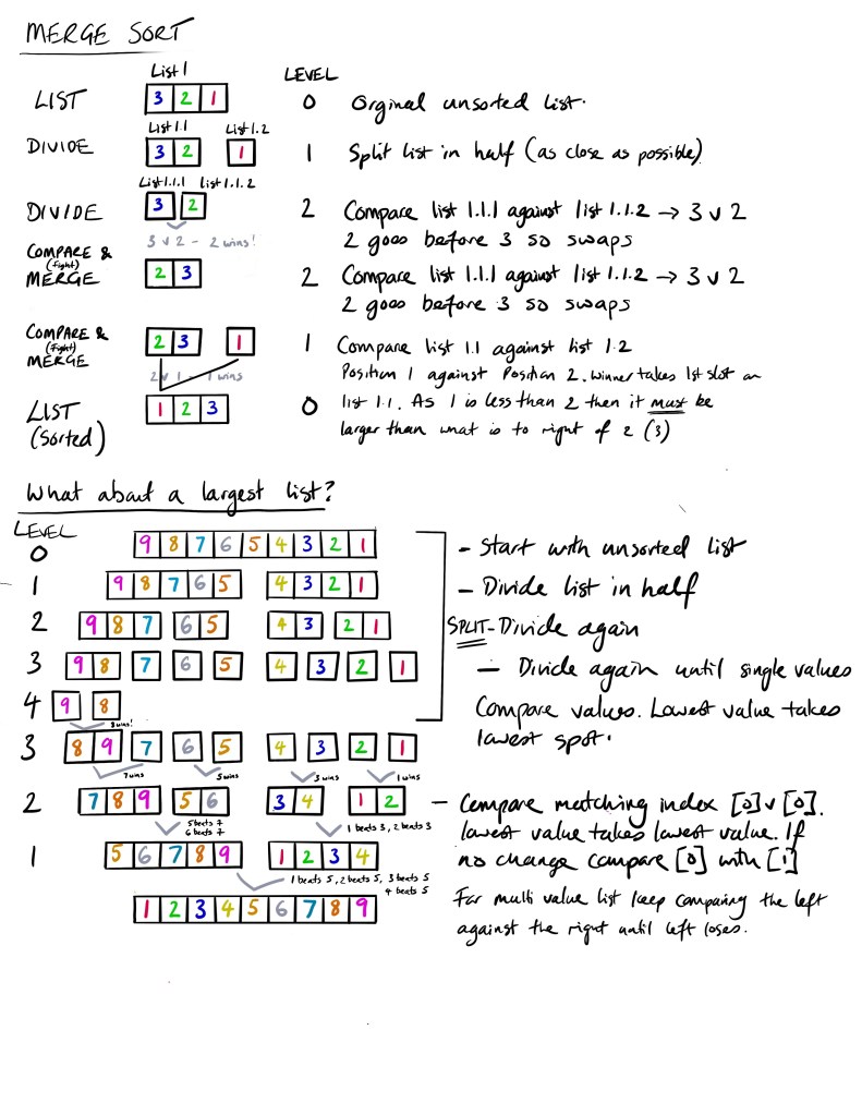
Although the merge sort and the bubble sort both get to the same place the merge sort works by two main loops: one to split the original list and one to compare and rebuild into a sorted list. Having the ability to split very long lists into single components can be done very quickly as it’s just splitting a list in half. Once the division is done then it’s simply a case of merging them back together. This can be even more efficient if the merging can be done by more than one processor in effecting solving the the sorting through parallel processing which is tricky with the bubble sort as we have only one list to work through.
Insertion Sort
The final sort we are going to look at is one that is probably the most obvious in a human logical way. The insertion sort is similar to the bubble sort but, sort of, works in the opposite direction. Whilst the bubble sort compares a pair of values and swaps them if needed until the value meets something greater the insertion sort takes a value and compares it items lower in the list until it meets a value lower or the end of the list.
An analogy would be set of cards. To sort them you place down the first card and then the second and compare the second with the first (not the first with the second even though it has the same effect). If the second is less than the first swap. Then pick the third card and compare to card 2 – is it a swap? Yes – compare with position 1 – is it a swap? No – place in position 2. The key thing with an insertion sort is that once the list is sorted with the card picked up you move to the next one and compare with values lower. To do this we hold the value we are sorting in our hand or in a temporary list of one. This value is not placed back into the list until it has found its place.
Let’s look at a list of three values to see how it works
List_1 = [2,3,1]
Length of list = 3
# check from left to right the lowest value. If lower swap with higher value and compare with values lower down the list

Check 1st position (compare position [1] to the left. Hold value in position [1])
Starting list [2,3,1]
Is value at index [1] less than the value on its left [0]?
[0] [1] [2]
 2   3   1
No - leave values at [0] to [1]
Are there more values in the list to compare?
No
End

Check 3rd position (compare position [2] to the left)
Starting list [2,3,1]

Is value at index [2] less than the value on its left [1]?
[0] [1] [2]
 2   3   1
Yes - move values at [1] to [2] (still hold original value at [1]
Are there more values in the list to compare?
Yes
Is value at index [1] less than the value on its left [0]?
Yes - move values at [0] to [1]
Are there more values in the list to compare?
No
Insert value original at position [2] to position [0]

Final list [1,2,3]

End
The simplest of the insert swap is that you sort as you go so you don’t need to iterate back to the start again like you do with a bubble sort. The disadvantage is you have to spend the time checking a swapped value all the way back but the overall overhead is the same.
Bubble, merge and insertion are the three major sorting algorithms to know especially for GCSE computer science.
Searching
All this talk of lists makes us think what do we actually do with them. We normally store items in a list so we can find them again or count them to see what we have collected. Counting we have done by simply finding the length of the list. For searching this is more fun and where algorithms are needed due to the repetitive nature of searching lists in a methodical manner.
There are two algorithms to learn when it comes to search: 1) linear for those lists we could (can not) sort and 2) binary for those list we are sorted or ‘ordered’.
Linear Search
Linear search is something we do when we know the list is short and we know the thing we are look for is in the list. Imagine you are working in a restaurant that has taken bookings for the 8pm slot in the order in which customers booked. When a customer turns up and asks for a table you would start at the top of the list and work your way down until you find the name of the person or tell them they don’t have a reservation. This is a linear search as you are checking every value until you get to the value that you are looking for. If the value is found you can cross them out making the next search easier and just in case you have multiple people of the same name. The code compared to the sort algorithms is straight forward.
def name_search(list_of_guests, N, find_name):
#find a guest from a list of guests
    for i in range(0, N):
        if (list_of_guests[i] == find_name):
            return i
    return -1

if __name__ == "__main__":
    list_of_guests = ['jones', 'smith']
    find_name = input("Enter name: ")
    N = len(list_of_guests)

    # Function call
    result = name_search(list_of_guests, N, find_name.lower())

    if(result == -1):
        print("I'm sorry. We don't have your name. Please book again.")
    else:
        result = result + 1
        print("We have your name. You are on table ", result)
In the code above we have created a function that takes in three arguments: list of guests, the number of elements in the list, and the name we are looking for. There is then a loop that goes through the list of names (list_of_guests) against the name we are looking for (find_name). If it finds the name (i equals find_name) then it return the value of the index in the list. If it does not then it returns the value -1.
To run the function we load in our list which is hard coded in the example but could be pulled from somewhere else and then get the person to enter the name they think is on the list. We also set the length of the list. With this all set we are ready to run the function called name_search which when run will return a value to the value called ‘return’. Before we do that we do a little bit of formatting by changing the name to lower case (find_name.lower()) as the user may enter Jones or jones or JONES or even jONES. We don’t have to do that do ideally we are formatting outside of the function instead of letting things in and then processing.
The function then runs and either finds the name or does not. If it does then it returns a nice message confirming they have the name and what table the guests are at (we could something fancy here are get the actual table but keeping it simple. If the name is not found then the guest is asked to try and book again. Nice and simple.
Where the linear search struggles is very long lists – imagine your name in a phone book. If we started at the As and went all the way down to the Zs (or the alphabet of your choice) then fine if the list is small or if the name is Aaron. With longer lists we need to have a more logically approach and this is where the next search algorithm comes in.
Binary Search
Binary search sounds maths and technical – “execute a binary search to find the name!” – but we do it all the time when we are presented with an ordered list. With binary search we take an ordered numbered list or we apply an index to make it an ordered number list or array, define the middle value by dividing the list by 2 (round up if a fraction) and compare this value to the number we are searching for.
There are three things that could happen after we have defined the middle value:
- Search value matches middle value – stop the search
- Search value is less than middle value – keep searching to the left of the middle value
- Search value is greater than the middle value – keep searching to the right of the middle value.
- Define the new middle value of the halved list
We then repeat this sequence until we chop the list down to a single value. We do something like this when we are trying to find something in a dictionary (a physical one – they still exist) – we open the book roughly where we thing the word would could be. If we don’t find it we split the section a bit closer and then closer until we find the page we are after.
A search for a letter in an alphabet is a perfect example of using the binary search. Let’s say we are looking for the letter ‘s’. First thing we need to do is index the order we want to the list to be in (this makes it an array but let’s just use list for the layman). An index alphabet looks like the following. We’ve marked out the letter ‘s’ at position 19. A quick note – the list could start at 0 rather than 1 – it doesn’t matter.
| i | 1 | 2 | 3 | 4 | 5 | 6 | 7 | 8 | 9 | 10 | 11 | 12 | 13 | 14 | 15 | 16 | 17 | 18 | 19 | 20 | 21 | 22 | 23 | 24 | 25 | 26 |
| v | a | b | c | d | e | f | g | h | i | j | k | l | m | n | o | p | q | r | s | t | u | v | w | x | y | z |
Let’s go through the binary search algorithm.
Step 1. Find the middle value by taking the highest value from the lowest then divide by 2 (if a fraction 0.5 round up).
(high – low) / 2 round up to whole number => (26 -1)/2 =12.5 => 13
Step 2. Check the middle value (13) against the search value (19)
i) If search value = middle value => search value found. Search complete.
(19 = 13 False)
ii) else If search value < middle value => search value is less than middle value, discard all values equal to or greater than middle value. Keep everything less than middle value.
(19 < 13 False)
iii) else search value > middle value => search value is more than middle value, discard all values equal to greater found. Search complete. Keep everything more than middle value.
(19 > 13 True)
| i | 1 | 2 | 3 | 4 | 5 | 6 | 7 | 8 | 9 | 10 | 11 | 12 | 13 | 14 | 15 | 16 | 17 | 18 | 19 | 20 | 21 | 22 | 23 | 24 | 25 | 26 |
| v | a | b | c | d | e | f | g | h | i | j | k | l | m | n | o | p | q | r | s | t | u | v | w | x | y | z |
| d | i | s | c | a | r | – | – | – | – | – | – | – | k | e | e | p | . | . | . | . | . | . | . | . | . |
This is our new search list. Hopefully you can see that the values greater than the middle value are removed or deleted from the list – it’s still there but we don’t be searching that part any more. We repeat there process as before with one additional step.
Step 1 – Find the middle. Same as before (high – low) / 2 => (26 – 14) /2 = 6. To find the middle we need to add the index of the list we are not searching which is the low value => 14 + 6 = 20 – marked in blue in the table below.
| i | 1 | 2 | 3 | 4 | 5 | 6 | 7 | 8 | 9 | 10 | 11 | 12 | 13 | 14 | 15 | 16 | 17 | 18 | 19 | 20 | 21 | 22 | 23 | 24 | 25 | 26 |
| v | a | b | c | d | e | f | g | h | i | j | k | l | m | n | o | p | q | r | s | t | u | v | w | x | y | z |
Step 2 – Exactly the same as before … check the middle value (20) against the search value (19)
i) If search value = middle value => search value found. Search complete.
(19 = 20 False) [so close!]
ii) else If search value < middle value => search value is less than middle value, discard all values equal to or greater than middle value. Keep everything less than middle value.
(19 < 20 True)
iii) else search value > middle value => search value is more than middle value, discard all values equal to greater found. Search complete. Keep everything more than middle value.
(19 > 20 False)
This time we remove everything less than the mid value (20) as the search value is in this section. We have split the list from 26 to 6 in two steps and that is the power of the binary search. But we’ve not done. Let’s keep going.
| i | 1 | 2 | 3 | 4 | 5 | 6 | 7 | 8 | 9 | 10 | 11 | 12 | 13 | 14 | 15 | 16 | 17 | 18 | 19 | 20 | 21 | 22 | 23 | 24 | 25 | 26 |
| v | a | b | c | d | e | f | g | h | i | j | k | l | m | n | o | p | q | r | s | t | u | v | w | x | y | z |
Step 1 – Find the middle. High = 19, Low = 14
((high – low) / 2) + low => ((19 – 14) / 2) + 14 = (5/2) + 14 = 17 (round up)
| i | 1 | 2 | 3 | 4 | 5 | 6 | 7 | 8 | 9 | 10 | 11 | 12 | 13 | 14 | 15 | 16 | 17 | 18 | 19 | 20 | 21 | 22 | 23 | 24 | 25 | 26 |
| v | a | b | c | d | e | f | g | h | i | j | k | l | m | n | o | p | q | r | s | t | u | v | w | x | y | z |
Step 2 – Check the middle value (17) against the search value (19)
i) If search value = middle value => search value found. Search complete.
(19 = 17 False)
ii) else If search value < middle value => search value is less than middle value, discard all values equal to or greater than middle value. Keep everything less than middle value.
(19 < 17 False)
iii) else search value > middle value => search value is more than middle value, discard all values equal to greater found. Search complete. Keep everything more than middle value.
(19 > 17 True)
| i | 1 | 2 | 3 | 4 | 5 | 6 | 7 | 8 | 9 | 10 | 11 | 12 | 13 | 14 | 15 | 16 | 17 | 18 | 19 | 20 | 21 | 22 | 23 | 24 | 25 | 26 |
| v | a | b | c | d | e | f | g | h | i | j | k | l | m | n | o | p | q | r | s | t | u | v | w | x | y | z |
Getting close – down to two values. Keep going on this round.
Step 1 – Find the middle. High = 19, Low = 18
((high – low) / 2) + low => ((19 – 18) / 2) + 18 = (1/2) + 18 = 19 (round up)
| i | 1 | 2 | 3 | 4 | 5 | 6 | 7 | 8 | 9 | 10 | 11 | 12 | 13 | 14 | 15 | 16 | 17 | 18 | 19 | 20 | 21 | 22 | 23 | 24 | 25 | 26 |
| v | a | b | c | d | e | f | g | h | i | j | k | l | m | n | o | p | q | r | s | t | u | v | w | x | y | z |
Step 2 – Check the middle value (19) against the search value (19)
i) If search value = middle value => search value found. Search complete.
(19 = 19 True) – FOUND VALUE!
ii) else If search value < middle value => search value is less than middle value, discard all values equal to or greater than middle value. Keep everything less than middle value.
(19 < 19 False)
iii) else search value > middle value => search value is more than middle value, discard all values equal to greater found. Search complete. Keep everything more than middle value.
(19 > 19 True)
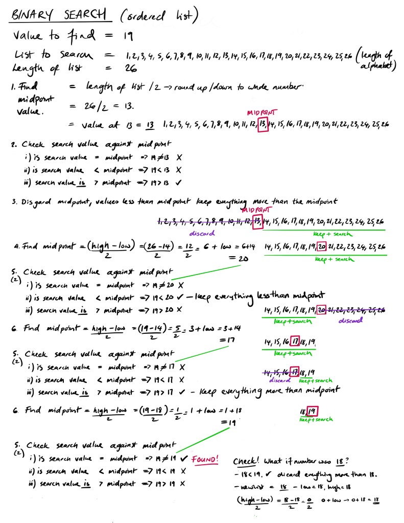
From a list of 26 it took four rounds to find the value 19 which corresponds to the letter ‘s’. Nice. Too try and illustrate this check out the picture below which looks to explain the binary search like just did plus a little extra on what to do if the number was 18!
Turning this into an algorithm is straight forward enough. Below is the python3 for the above description. The code uses a while loop to run as long as low number of the array is not less than or equal to the high number of the array.
# Python3 code to implement iterative Binary Search. (copied and changed from Geeks for Geeks - ref https://www.geeksforgeeks.org/binary-search/)


# function that takes the incoming array, the lowest index of the array, the highest index in the array, and the number being searching for

def binarySearch(arr, low, high, x):
# arr is the array to search, low is the lowest index value of the array, high is the highest index value of the array, x is the value been search for

    while low <= high:

        mid = ((high - low) // 2) + low

        # Check if x is present at mid point then stop and return the mid value
        if arr[mid] == x:
            return mid

        # If x is greater, ignore left half side only search right side
        elif arr[mid] < x:
            low = mid + 1.    # set the new low to be 1 higher than current mid point

        # If x is smaller, ignore right half and only search left side
        else:
            high = mid - 1.   # set the new high to be 1 lower than the current mid point

    # If we reach here, then the element
    # was not present
    return -1


# Test Code
arr = [1,2,3,4,5,6,7,8,9,10,11,12,13,14,15,16,17,18,19,20,21,22,23,25,26]
x = 10

    # Function call
    result = binarySearch(arr, 0, len(arr)-1, x) #load the function with the arr, the low value (0), high value, and search value
    if result != -1:
        print("Element is present at index", result)
    else:
        print("Element is not present in array")
Summary
A very long page to cover the art of computer thinking and some of the fundamentals of algorithms. If you understand it all then don’t worry. At this point it is all about appreciating that writing computer programs takes some thought but by carefully considering what the problem is and how a solution would work allows the problem to be broken down into inputs, processes, and outputs where the processes can be repeating/reusable blocks of code called algorithms.
Start: Algorithms | > Next: Programming Fundamentals
